📍 Pick Points#
Extract Model Grid Data at Specific Points with Herbie#
Extract weather model data at point locations | Interpolate gridded data | Sample NWP grids
Herbie’s pick_points xarray accessor extracts values from weather and climate model grids at specific latitude/longitude locations. Whether you need to sample HRRR, GFS, or other numerical weather prediction (NWP) model output at station locations, city coordinates, or arbitrary points, this tool provides efficient nearest-neighbor and distance-weighted interpolation.

What you’ll learn: Extract and Interpolate Model Data#
In this tutorial, you’ll learn how to:
Extract point values from gridded model data (HRRR, GFS, NAM, etc.)
Sample weather models at specific latitude/longitude coordinates
Work with both regular grids (lat/lon) and curvilinear grids (Lambert Conformal, polar stereographic)
Use nearest-neighbor vs distance-weighted interpolation methods
Create time series from model forecasts at station locations
Extract vertical profiles (model soundings) at points
Interpolate GRIB2 data to observation sites
Optimize performance for extracting hundreds or thousands of points
Cache spatial indices (BallTree) for faster repeated queries
Common Use Cases#
Compare model output to weather station observations
Extract forecast data for specific cities or locations
Create model soundings at radiosonde sites
Sample gridded forecasts along flight paths or trajectories
Validate NWP models against point measurements
Extract model data for machine learning training datasets
Requirements: This tutorial requires the scikit-learn package for spatial indexing:
pip install scikit-learn
# or install with all Herbie extras
pip install 'herbie-data[extras]'
How it Works: Spatial Indexing with BallTree#
Herbie uses scikit-learn’s BallTree algorithm with the haversine formula for accurate nearest-neighbor queries on Earth’s spherical surface. This approach works for any model grid projection without requiring coordinate transformations.
Advantages over other methods:#
✅ Works with curvilinear/projected grids (HRRR, NAM, WRF)
✅ Handles longitude convention differences (0-360° vs ±180°)
✅ Returns distance to nearest grid points (great-circle distance in km)
✅ Supports k-nearest neighbors for interpolation and uncertainty quantification
✅ Fast queries even for thousands of points
✅ No coordinate transformation required
Background: When to Use Pick Points#
For regular latitude-longitude grids (e.g., GFS, IFS), you could use xarray’s advanced indexing to select your points of interest. However, pick_points is necessary when:
Curvilinear grids: Models like HRRR use Lambert Conformal or other map projections
Longitude conventions differ: Model uses [0, 360) but your points are in [-180, 180)
Distance matters: You need to know how far the nearest grid point is from your location
Multiple neighbors: You want k-nearest points for interpolation or statistics
Performance: Extracting many points at once (spatial indexing is very fast)
Batch processing: Repeatedly querying the same grid (BallTree caching)
Development History: Why I Built This
Picking values at nearest-neighbor points in a curvilinear grid has been one of my longstanding challenges. In November 2019, I asked How to select the nearest lat/lon location with multi-dimension coordinates on Stack Overflow, which has had over 28k views. My initial solution found the minimum distance between points and grid cells, but it didn’t scale well for many points.
I iterated through several approaches:
Previous approach (deprecated): ds.herbie.nearest_points used MetPy’s assign_y_x to transform coordinates to the model’s projection (e.g., Lambert Conformal for HRRR), then selected nearest neighbors. This worked but required Cartopy coordinate transformations, and not all datasets have sufficient projection metadata.
Current approach: Using BallTree with haversine distance:
✅ No coordinate transformation needed
✅ Can extract k-nearest neighbors
✅ Returns actual distances (km) using haversine formula
✅ Supports inverse-distance weighted interpolation
✅ Much faster for bulk queries
I later discovered the xoak package, which also uses BallTree for nearest neighbors.
Getting Started#
To use Herbie’s xarray accessors, just import Herbie (the accessor registers automatically):
[1]:
import warnings

import matplotlib.pyplot as plt
import numpy as np
import pandas as pd
import xarray as xr

import herbie
from herbie import FastHerbie, Herbie
A Very Simple Demonstration#
First, I’ll show how Herbie extracts nearest points from a simple grid. Let’s make a 3x3 xarray Dataset with latitude/longitude coordinates and then extract data nearest two points of interest.
[2]:
# Create a 3x3 xarray dataset
ds = xr.Dataset(
    {"a": (["latitude", "longitude"], [[0, 1, 2], [0, 1, 0], [0, 0, 0]])},
    coords={
        "latitude": (["latitude"], [44, 45, 46]),
        "longitude": (["longitude"], [-99, -100, -101]),
    },
)
ds
[2]:
<xarray.Dataset> Size: 120B
Dimensions:    (latitude: 3, longitude: 3)
Coordinates:
  * latitude   (latitude) int64 24B 44 45 46
  * longitude  (longitude) int64 24B -99 -100 -101
Data variables:
a (latitude, longitude) int64 72B 0 1 2 0 1 0 0 0 0The points you want to extract must be given as a Pandas DataFrame with columns latitude and longitude given in degrees.
[3]:
# We want to pick data closest to two points
points = pd.DataFrame(
    {
        "longitude": [-100.25, -99.4],
        "latitude": [44.25, 45.4],
    }
)
points
[3]:
| longitude | latitude | |
|---|---|---|
| 0 | -100.25 | 44.25 |
| 1 | -99.40 | 45.40 |
Now we can pick the nearest grid points with the custom Herbie xarray accessor.
Note
method='nearest'is the default behavior.
[4]:
# Pick the value nearest the requested points
matched = ds.herbie.pick_points(points, method="nearest")
matched
WARNING: BallTree caching disabled - tree_name not specified.
         Provide tree_name parameter to enable caching.
INFO: 🌱 Growing new BallTree...🌳 Complete in 0.01s
[4]:
<xarray.Dataset> Size: 96B
Dimensions:              (point: 2)
Coordinates:
    latitude             (point) int64 16B 44 45
    longitude            (point) int64 16B -100 -99
    point_grid_distance  (point) float64 16B 34.22 54.41
    point_longitude      (point) float64 16B -100.2 -99.4
    point_latitude       (point) float64 16B 44.25 45.4
Dimensions without coordinates: point
Data variables:
a (point) int64 16B 1 0Alternatively, we can get the inverse-distance weighted mean of the 4 nearest points.
[5]:
# Distance weighted mean
matched_w = ds.herbie.pick_points(points, method="weighted")
matched_w
WARNING: BallTree caching disabled - tree_name not specified.
         Provide tree_name parameter to enable caching.
INFO: 🌱 Growing new BallTree...🌳 Complete in 0.00s
[5]:
<xarray.Dataset> Size: 240B
Dimensions:              (point: 2, k: 4)
Coordinates:
    point_longitude      (point) float64 16B -100.2 -99.4
    point_latitude       (point) float64 16B 44.25 45.4
    latitude             (k, point) int64 64B 44 45 44 45 45 46 45 46
    longitude            (k, point) int64 64B -100 -99 -101 ... -99 -101 -100
    point_grid_distance  (k, point) float64 64B 34.22 54.41 66.0 ... 102.4 81.38
Dimensions without coordinates: point, k
Data variables:
    a                    (point) float64 16B 1.082 0.2588
Attributes:
    pick_point_method:  weighted
pick_point_k: 4Understanding the Output#
The returned Dataset includes several useful coordinates:
point_latitude,point_longitude: Your requested coordinatespoint_grid_distance: Distance (km) to the nearest grid pointlatitude,longitude: The actual grid point coordinatesAny additional columns from your points DataFrame (e.g.,
point_stid)
The point dimension indexes your requested points.
That’s a lot of info to digest. Let’s visualize what we have done with the following figure:
[6]:
fig, axes = plt.subplots(1, 2, figsize=[13, 5])
for p, ax in zip(matched_w.point, axes):
    zz = matched.sel(point=p)

    # Plot grid
    ax.pcolormesh(
        ds.longitude, ds.latitude, ds.a, edgecolor="1", lw=1, cmap="Pastel2_r"
    )
    x, y = np.meshgrid(ds.longitude, ds.latitude)
    x = x.flatten()
    y = y.flatten()
    ax.scatter(x, y, facecolor="tab:red", edgecolor="tab:red", s=100, zorder=100)

    # Plot requested point
    ax.scatter(
        zz.point_longitude,
        zz.point_latitude,
        color="yellow",
        ec="k",
        marker="p",
        s=300,
        zorder=100,
    )
    for i in ds.latitude:
        for j in ds.longitude:
            z = ds.sel(latitude=i, longitude=j)
            ax.text(j, i, f"\na={z.a.item()}", ha="center", va="top")

    # Plot path to nearest point and distance
    # for i, j in zip(x, y):
    #    ax.plot([i, point.longitude.values[0]], [j, point.latitude.values[0]])
    for i in matched_w.k:
        if i == 0:
            kwargs = dict(lw=2, color="k", ls="--")
        else:
            kwargs = dict(color=".5", ls="--")
        z = matched_w.sel(k=i, point=p)
        ax.plot(
            [z.longitude, z.point_longitude], [z.latitude, z.point_latitude], **kwargs
        )
        ax.text(
            z.longitude,
            z.latitude,
            f"  {z.point_grid_distance.item():.1f} km",
            va="center",
            fontweight="bold",
        )
    ax.set_xticks(ds.longitude)
    ax.set_yticks(ds.latitude)
    ax.set_xlabel("Longitude")
    ax.set_ylabel("Latitude")
    ax.set_title(f"Point={p.item()}", loc="left", fontsize="xx-large")
    ax.set_title(
        f"nearest value:  $a={zz.a.item():.2f}$\nweighted mean:  $a={z.a.item():.2f}$",
        loc="right",
    )
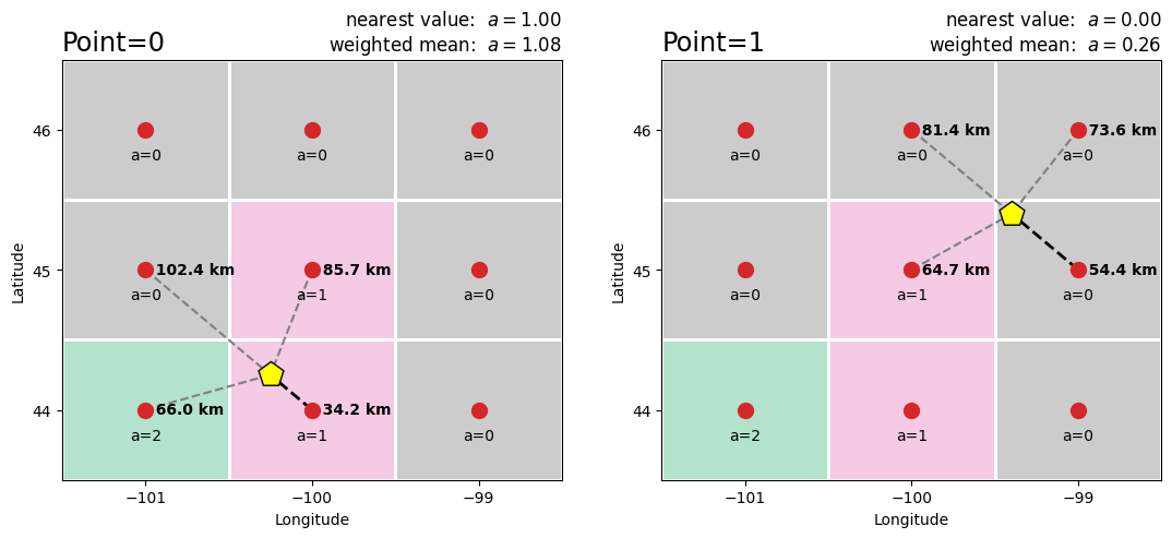
The yellow pentagon is the requested point. The grid’s nearest-neighbor point is connected by a thick dashed line. The three other nearest neighbors used to compute the distance-weighted mean are connected by a thin dashed line.
Summary: From a simple 2D Dataset with latitude and longitude coordinates, we got the nearest value for two points of interest. We also compute the inverse-distance weighted mean from the four grids nearest our point of interest.
Pick points from HRRR data#
The above is nice, but you might say, “Yeah, but you can already select data from a grid using xarray advanced selection.” That is true, but it does not work for models with curvilienar grids, like the HRRR model.
Here is a demonstration using real HRRR data.
[7]:
H = Herbie("2024-03-01", model="hrrr")
ds = H.xarray(":(?:TMP|DPT):2 m")
ds
✅ Found ┊ model=hrrr ┊ product=sfc ┊ 2024-Mar-01 00:00 UTC F00 ┊ GRIB2 @ aws ┊ IDX @ local
[7]:
<xarray.Dataset> Size: 46MB
Dimensions:              (y: 1059, x: 1799)
Coordinates:
    time                 datetime64[ns] 8B 2024-03-01
    step                 timedelta64[ns] 8B 00:00:00
    heightAboveGround    float64 8B 2.0
    latitude             (y, x) float64 15MB 21.14 21.15 21.15 ... 47.85 47.84
    longitude            (y, x) float64 15MB 237.3 237.3 237.3 ... 299.0 299.1
    valid_time           datetime64[ns] 8B 2024-03-01
    gribfile_projection  object 8B None
Dimensions without coordinates: y, x
Data variables:
    t2m                  (y, x) float32 8MB 292.5 292.5 292.4 ... 266.8 266.8
    d2m                  (y, x) float32 8MB 287.3 287.2 287.2 ... 262.2 262.2
Attributes:
    GRIB_edition:            2
    GRIB_centre:             kwbc
    GRIB_centreDescription:  US National Weather Service - NCEP
    GRIB_subCentre:          0
    Conventions:             CF-1.7
    institution:             US National Weather Service - NCEP
    model:                   hrrr
    product:                 sfc
    description:             High-Resolution Rapid Refresh - CONUS
    remote_grib:             https://noaa-hrrr-bdp-pds.s3.amazonaws.com/hrrr....
    local_grib:              /home/blaylock/data/hrrr/20240301/subset_e0ef89f...
search: :(?:TMP|DPT):2 mLet’s extract the data from some points with some fruit-themed station id names.
[8]:
points = pd.DataFrame(
    {
        "latitude": np.linspace(44, 45.5, 5),
        "longitude": np.linspace(-100, -101, 5),
        "stid": ["McIntosh", "Golden", "Fuji", "Gala", "Honeycrisp"],
    }
)
points
[8]:
| latitude | longitude | stid | |
|---|---|---|---|
| 0 | 44.000 | -100.00 | McIntosh |
| 1 | 44.375 | -100.25 | Golden |
| 2 | 44.750 | -100.50 | Fuji |
| 3 | 45.125 | -100.75 | Gala |
| 4 | 45.500 | -101.00 | Honeycrisp |
[9]:
%%time
matched = ds.herbie.pick_points(points)
matched
CPU times: user 330 ms, sys: 414 ms, total: 744 ms
Wall time: 764 ms
[9]:
<xarray.Dataset> Size: 320B
Dimensions:              (point: 5)
Coordinates:
    time                 datetime64[ns] 8B 2024-03-01
    step                 timedelta64[ns] 8B 00:00:00
    heightAboveGround    float64 8B 2.0
    latitude             (point) float64 40B 43.99 44.37 44.76 45.13 45.5
    longitude            (point) float64 40B 260.0 259.8 259.5 259.3 259.0
    valid_time           datetime64[ns] 8B 2024-03-01
    gribfile_projection  object 8B None
    point_grid_distance  (point) float64 40B 0.8515 1.07 1.611 1.41 1.318
    point_latitude       (point) float64 40B 44.0 44.38 44.75 45.12 45.5
    point_longitude      (point) float64 40B -100.0 -100.2 -100.5 -100.8 -101.0
    point_stid           (point) object 40B 'McIntosh' 'Golden' ... 'Honeycrisp'
Dimensions without coordinates: point
Data variables:
    t2m                  (point) float32 20B 288.0 286.7 286.1 282.3 284.8
    d2m                  (point) float32 20B 268.8 271.8 270.5 274.1 270.5
Attributes:
    GRIB_edition:            2
    GRIB_centre:             kwbc
    GRIB_centreDescription:  US National Weather Service - NCEP
    GRIB_subCentre:          0
    Conventions:             CF-1.7
    institution:             US National Weather Service - NCEP
    model:                   hrrr
    product:                 sfc
    description:             High-Resolution Rapid Refresh - CONUS
    remote_grib:             https://noaa-hrrr-bdp-pds.s3.amazonaws.com/hrrr....
    local_grib:              /home/blaylock/data/hrrr/20240301/subset_e0ef89f...
search: :(?:TMP|DPT):2 mNotice that a BallTree object for the HRRR model was saved with the name <model_name>_<x_dim>_<y_dim>.pkl in the directory you save Herbie data. This is done so it can be loaded more quickly next time you extract points from this grid.
In the next cell I run the same command, and it uses the cached tree instead.
[10]:
%%time
matched = ds.herbie.pick_points(points)
matched
CPU times: user 523 ms, sys: 241 ms, total: 764 ms
Wall time: 760 ms
[10]:
<xarray.Dataset> Size: 320B
Dimensions:              (point: 5)
Coordinates:
    time                 datetime64[ns] 8B 2024-03-01
    step                 timedelta64[ns] 8B 00:00:00
    heightAboveGround    float64 8B 2.0
    latitude             (point) float64 40B 43.99 44.37 44.76 45.13 45.5
    longitude            (point) float64 40B 260.0 259.8 259.5 259.3 259.0
    valid_time           datetime64[ns] 8B 2024-03-01
    gribfile_projection  object 8B None
    point_grid_distance  (point) float64 40B 0.8515 1.07 1.611 1.41 1.318
    point_latitude       (point) float64 40B 44.0 44.38 44.75 45.12 45.5
    point_longitude      (point) float64 40B -100.0 -100.2 -100.5 -100.8 -101.0
    point_stid           (point) object 40B 'McIntosh' 'Golden' ... 'Honeycrisp'
Dimensions without coordinates: point
Data variables:
    t2m                  (point) float32 20B 288.0 286.7 286.1 282.3 284.8
    d2m                  (point) float32 20B 268.8 271.8 270.5 274.1 270.5
Attributes:
    GRIB_edition:            2
    GRIB_centre:             kwbc
    GRIB_centreDescription:  US National Weather Service - NCEP
    GRIB_subCentre:          0
    Conventions:             CF-1.7
    institution:             US National Weather Service - NCEP
    model:                   hrrr
    product:                 sfc
    description:             High-Resolution Rapid Refresh - CONUS
    remote_grib:             https://noaa-hrrr-bdp-pds.s3.amazonaws.com/hrrr....
    local_grib:              /home/blaylock/data/hrrr/20240301/subset_e0ef89f...
search: :(?:TMP|DPT):2 mYou may want to swap the dimensions to use the point_stid coordinate as the dimension instead. Doing this makes it possible to select data by station ID instead of point index.
[11]:
matched = matched.swap_dims({"point": "point_stid"})
matched.sel(point_stid="Honeycrisp")
[11]:
<xarray.Dataset> Size: 128B
Dimensions:              ()
Coordinates:
    time                 datetime64[ns] 8B 2024-03-01
    step                 timedelta64[ns] 8B 00:00:00
    heightAboveGround    float64 8B 2.0
    latitude             float64 8B 45.5
    longitude            float64 8B 259.0
    valid_time           datetime64[ns] 8B 2024-03-01
    gribfile_projection  object 8B None
    point_grid_distance  float64 8B 1.318
    point_latitude       float64 8B 45.5
    point_longitude      float64 8B -101.0
    point_stid           <U10 40B 'Honeycrisp'
Data variables:
    t2m                  float32 4B 284.8
    d2m                  float32 4B 270.5
Attributes:
    GRIB_edition:            2
    GRIB_centre:             kwbc
    GRIB_centreDescription:  US National Weather Service - NCEP
    GRIB_subCentre:          0
    Conventions:             CF-1.7
    institution:             US National Weather Service - NCEP
    model:                   hrrr
    product:                 sfc
    description:             High-Resolution Rapid Refresh - CONUS
    remote_grib:             https://noaa-hrrr-bdp-pds.s3.amazonaws.com/hrrr....
    local_grib:              /home/blaylock/data/hrrr/20240301/subset_e0ef89f...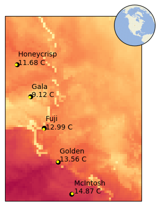
search: :(?:TMP|DPT):2 mNow let’s plot each point on a map with the value at the nearest grid point.
[12]:
from herbie.toolbox import EasyMap, ccrs, pc

ax = EasyMap(crs=ds.herbie.crs).ax
ax.pcolormesh(
    ds.longitude,
    ds.latitude,
    ds.t2m,
    cmap="Spectral_r",
    vmax=290,
    vmin=270,
    transform=pc,
)

for i in matched.point_stid:
    z = matched.sel(point_stid=i)
    ax.scatter(z.longitude, z.latitude, color="k", transform=pc)
    ax.scatter(
        z.point_longitude, z.point_latitude, color="yellow", marker=".", transform=pc
    )
    ax.text(
        z.point_longitude,
        z.point_latitude,
        f" {z.point_stid.item()}\n {z.t2m.item() - 273.15:.2f} C",
        transform=pc,
    )
ax.set_extent([-101, -99, 44, 46], crs=pc)
ax.EasyMap.INSET_GLOBE()
ax.adjust_extent()
[12]:
(-289442.889311017, -108684.3334160587, 605320.486730601, 849853.0858732163)
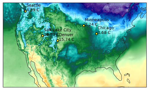
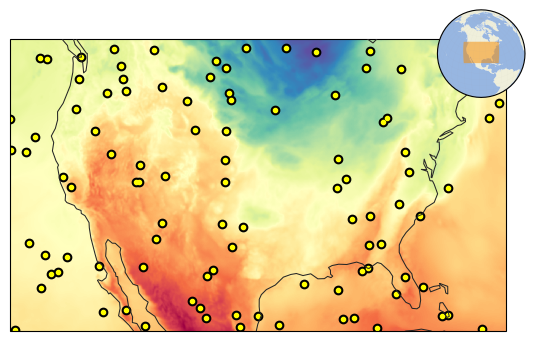
Here is another example with several cities
[13]:
points = pd.DataFrame(
    {
        "latitude": [40.7608, 41.8781, 39.7392, 44.9778, 47.6062],
        "longitude": [-111.8910, -87.6298, -104.9903, -93.2650, -122.3321],
        "stid": ["Salt Lake City", "Chicago", "Denver", "Minneapolis", "Seattle"],
        "elevation": [1288, 182, 1655, 264, 56],  # Optional: add metadata
    }
)

# ---------------
# Pick the points
matched = ds.herbie.pick_points(points)

# -------------
# Make the plot

from herbie.paint import NWSTemperature

ax = EasyMap(crs=ds.herbie.crs).STATES().ax
ax.pcolormesh(
    ds.longitude,
    ds.latitude,
    ds.t2m - 273.15,
    **NWSTemperature.kwargs,
    transform=pc,
)

for i in matched.point:
    z = matched.sel(point=i)
    ax.scatter(z.longitude, z.latitude, color="k", transform=pc)
    ax.scatter(
        z.point_longitude, z.point_latitude, color="yellow", marker=".", transform=pc
    )
    ax.text(
        z.point_longitude,
        z.point_latitude,
        f" {z.point_stid.item()}\n {z.t2m.item() - 273.15:.2f} C",
        transform=pc,
    )
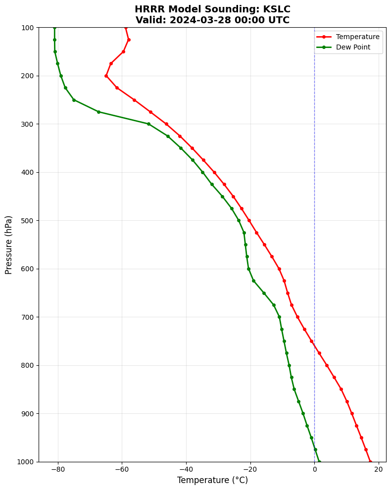
Pick Points: Sounding#
For vertical profiles, download all pressure levels and extract at a point. This creates a “model sounding” that can be compared to observations.
[14]:
# TODO: Get real sounding data to compare model data to.
[15]:
# Get all pressure level data
H = Herbie("2024-03-28 00:00", model="hrrr", product="prs")
ds = H.xarray("(?:DPT|TMP):[0-9]* mb", remove_grib=False)

slc_point = pd.DataFrame(
    {
        "latitude": [40.76],
        "longitude": [-111.876183],
        "stid": ["KSLC"],
    }
)

slc = ds.herbie.pick_points(slc_point)
slc
✅ Found ┊ model=hrrr ┊ product=prs ┊ 2024-Mar-28 00:00 UTC F00 ┊ GRIB2 @ aws ┊ IDX @ local
[15]:
<xarray.Dataset> Size: 704B
Dimensions:              (isobaricInhPa: 39, point: 1)
Coordinates:
    time                 datetime64[ns] 8B 2024-03-28
    step                 timedelta64[ns] 8B 00:00:00
  * isobaricInhPa        (isobaricInhPa) float64 312B 1e+03 975.0 ... 75.0 50.0
    latitude             (point) float64 8B 40.75
    longitude            (point) float64 8B 248.1
    valid_time           datetime64[ns] 8B 2024-03-28
    gribfile_projection  object 8B None
    point_grid_distance  (point) float64 8B 1.193
    point_latitude       (point) float64 8B 40.76
    point_longitude      (point) float64 8B -111.9
    point_stid           (point) object 8B 'KSLC'
Dimensions without coordinates: point
Data variables:
    t                    (isobaricInhPa, point) float32 156B ...
    dpt                  (isobaricInhPa, point) float32 156B ...
Attributes:
    GRIB_edition:            2
    GRIB_centre:             kwbc
    GRIB_centreDescription:  US National Weather Service - NCEP
    GRIB_subCentre:          0
    Conventions:             CF-1.7
    institution:             US National Weather Service - NCEP
    model:                   hrrr
    product:                 prs
    description:             High-Resolution Rapid Refresh - CONUS
    remote_grib:             https://noaa-hrrr-bdp-pds.s3.amazonaws.com/hrrr....
    local_grib:              /home/blaylock/data/hrrr/20240328/subset_0befd2f...
search: (?:DPT|TMP):[0-9]* mb[16]:
# Create a proper sounding plot
fig, ax = plt.subplots(figsize=(8, 10))

# Plot temperature and dewpoint
ax.plot(
    slc.t - 273.15,
    slc.isobaricInhPa,
    color="red",
    marker="o",
    linewidth=2,
    markersize=4,
    label="Temperature",
)
ax.plot(
    slc.dpt - 273.15,
    slc.isobaricInhPa,
    color="green",
    marker="o",
    linewidth=2,
    markersize=4,
    label="Dew Point",
)

# Format axes
ax.invert_yaxis()
ax.set_ylim(1000, 100)
ax.set_ylabel("Pressure (hPa)", fontsize=12)
ax.set_xlabel("Temperature (°C)", fontsize=12)
ax.set_title(
    f"HRRR Model Sounding: {slc.point_stid.item()}\n"
    f"Valid: {slc.valid_time.dt.strftime('%Y-%m-%d %H:%M UTC').item()}",
    fontsize=14,
    fontweight="bold",
)
ax.grid(True, alpha=0.3)
ax.legend(loc="upper right")

# Add reference lines
ax.axvline(0, color="blue", linestyle="--", alpha=0.5, linewidth=1)
plt.tight_layout()
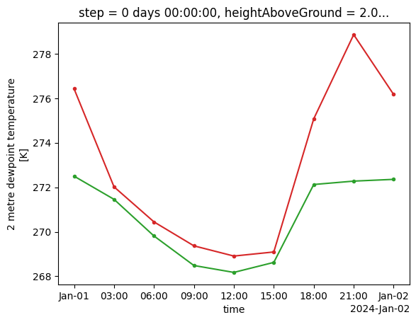
Pick Points: Timeseries#
[17]:
# TODO: Could demonstrate using FastHerbie here, if the kernel wouldn't crash (memory??)

i = []
for date in pd.date_range("2024-01-01", periods=9, freq="3h"):
    ds = Herbie(date).xarray("(?:DPT|TMP):2 m", remove_grib=False)
    i.append(
        ds.herbie.pick_points(
            pd.DataFrame(
                {
                    "latitude": [40.77069],
                    "longitude": [-111.96503],
                    "stid": ["KSLC"],
                }
            )
        )
    )
slc_ts = xr.concat(i, dim="valid_time")

slc_ts.t2m.plot(x="valid_time", marker=".", color="tab:red")
slc_ts.d2m.plot(x="valid_time", marker=".", color="tab:green")
✅ Found ┊ model=hrrr ┊ product=sfc ┊ 2024-Jan-01 00:00 UTC F00 ┊ GRIB2 @ aws ┊ IDX @ local
✅ Found ┊ model=hrrr ┊ product=sfc ┊ 2024-Jan-01 03:00 UTC F00 ┊ GRIB2 @ aws ┊ IDX @ local
✅ Found ┊ model=hrrr ┊ product=sfc ┊ 2024-Jan-01 06:00 UTC F00 ┊ GRIB2 @ aws ┊ IDX @ local
✅ Found ┊ model=hrrr ┊ product=sfc ┊ 2024-Jan-01 09:00 UTC F00 ┊ GRIB2 @ aws ┊ IDX @ local
✅ Found ┊ model=hrrr ┊ product=sfc ┊ 2024-Jan-01 12:00 UTC F00 ┊ GRIB2 @ aws ┊ IDX @ local
✅ Found ┊ model=hrrr ┊ product=sfc ┊ 2024-Jan-01 15:00 UTC F00 ┊ GRIB2 @ aws ┊ IDX @ local
✅ Found ┊ model=hrrr ┊ product=sfc ┊ 2024-Jan-01 18:00 UTC F00 ┊ GRIB2 @ aws ┊ IDX @ local
✅ Found ┊ model=hrrr ┊ product=sfc ┊ 2024-Jan-01 21:00 UTC F00 ┊ GRIB2 @ aws ┊ IDX @ local
✅ Found ┊ model=hrrr ┊ product=sfc ┊ 2024-Jan-02 00:00 UTC F00 ┊ GRIB2 @ aws ┊ IDX @ local
[17]:
[<matplotlib.lines.Line2D at 0x7d6e21642490>]
Benchmark#
Let’s benchmark picking different numbers of points to understand performance scaling when harvesting many points.
[18]:
import warnings

import matplotlib.pyplot as plt
import pandas as pd

from herbie import Herbie
from herbie.toolbox import EasyMap, ccrs, pc
[19]:
H = Herbie("2024-03-28 00:00", model="hrrr")
ds = H.xarray(r"TMP:\d* mb", remove_grib=False)
✅ Found ┊ model=hrrr ┊ product=sfc ┊ 2024-Mar-28 00:00 UTC F00 ┊ GRIB2 @ aws ┊ IDX @ local
Using the model’s own grid, I will generate 100 random samples to extract.
[20]:
def generate_test_points(ds, n):
    """Generate n random points from the model grid."""
    import random
    import string

    points = (
        ds[["latitude", "longitude"]]
        .to_dataframe()[["latitude", "longitude"]]
        .sample(n)
        .reset_index(drop=True)
    )
    points["stid"] = [
        "".join(random.choices(string.ascii_letters, k=8)) for _ in range(n)
    ]
    return points


points_self_100 = generate_test_points(ds, 100)
points_self_100
[20]:
| latitude | longitude | stid | |
|---|---|---|---|
| 0 | 29.718029 | 274.785946 | SkNxqxCY |
| 1 | 26.961634 | 255.333244 | DONsGClt |
| 2 | 47.380357 | 258.360720 | zBYYWqvk |
| 3 | 48.499379 | 236.466228 | PNKRmpQX |
| 4 | 37.763784 | 272.271894 | kgiLfUwp |
| ... | ... | ... | ... |
| 95 | 34.706803 | 275.869335 | RrdbpPvj |
| 96 | 25.423777 | 256.984473 | ELGWpzoF |
| 97 | 21.841066 | 285.435707 | iSCwEgju |
| 98 | 35.878342 | 285.655062 | UQBJvXzT |
| 99 | 45.136663 | 294.870079 | KYvNRgCr |
100 rows × 3 columns
[21]:
%%timeit
y1 = ds.herbie.pick_points(points_self_100)
542 ms ± 144 ms per loop (mean ± std. dev. of 7 runs, 1 loop each)
[22]:
%%timeit
y2 = ds.herbie.pick_points(points_self_100, method="weighted")
1.84 s ± 234 ms per loop (mean ± std. dev. of 7 runs, 1 loop each)
[23]:
%%timeit
# Try the deprecated `nearest_points` method which used MetPy
with warnings.catch_warnings():
    warnings.simplefilter("ignore")
    y3 = ds.herbie.nearest_points(points_self_100)
541 ms ± 76.5 ms per loop (mean ± std. dev. of 7 runs, 1 loop each)
[24]:
# Do I get the same answer for the old and new method?
y1 = ds.herbie.pick_points(points_self_100)
y2 = ds.herbie.pick_points(points_self_100, method="weighted")
y3 = ds.herbie.nearest_points(points_self_100)

all(y1.latitude == y3.latitude), all(y1.longitude == y3.longitude)
/home/blaylock/GITHUB/Herbie/src/herbie/nearest_points.py:109: UserWarning: More than one time coordinate present for variable  "t".
  ds = ds.metpy.assign_y_x()
[24]:
(True, True)
[25]:
%%time
ax = EasyMap(crs=ds.herbie.crs).ax

ax.pcolormesh(
    ds.longitude,
    ds.latitude,
    ds.isel(isobaricInhPa=0).t,
    cmap="Spectral_r",
    transform=pc,
)

ax.scatter(y1.longitude, y1.latitude, color="k", transform=pc)
ax.scatter(
    y1.point_longitude, y1.point_latitude, color="yellow", marker=".", transform=pc
)

ax.EasyMap.INSET_GLOBE()
CPU times: user 1.48 s, sys: 257 ms, total: 1.73 s
Wall time: 2.6 s
[25]:
<GeoAxes: label='inset_axes'>
Not bad. Less than half a second to extract 100 points from the HRRR grid.
Now let’s try even more…
[26]:
%%time

n_samples = (
    list(range(1, 10, 2)) + list(range(10, 100, 20)) + list(range(100, 1_000, 200))
    # + list(range(1_000, 10_000, 2_000))
    # + [100_000, 1_000_000]
)

times_pick_points_nearest = []
times_pick_points_weighted = []
times_nearest_points = []

with warnings.catch_warnings():
    warnings.simplefilter("ignore")

    for n in n_samples:
        points = generate_test_points(ds, n)

        timer = pd.Timestamp("now")
        _ = ds.herbie.nearest_points(points)
        times_nearest_points.append((pd.Timestamp("now") - timer).total_seconds())

        timer = pd.Timestamp("now")
        _ = ds.herbie.pick_points(points, method="nearest")
        times_pick_points_nearest.append((pd.Timestamp("now") - timer).total_seconds())

        timer = pd.Timestamp("now")
        _ = ds.herbie.pick_points(points, method="weighted")
        times_pick_points_weighted.append((pd.Timestamp("now") - timer).total_seconds())

        print(f"✓ Completed {n:,} points")

fig, ax = plt.subplots(figsize=(10, 6))
ax.plot(
    n_samples,
    times_pick_points_nearest,
    marker=".",
    lw=2,
    color="tab:blue",
    label="pick_points (nearest)",
)
ax.plot(
    n_samples,
    times_pick_points_weighted,
    marker=".",
    lw=2,
    color="tab:orange",
    label="pick_points (weighted)",
)
ax.plot(
    n_samples,
    times_nearest_points,
    marker=".",
    lw=1,
    color="k",
    ls="--",
    label="nearest_points (deprecated)",
)

ax.set_xscale("log")
ax.set_title("Performance: Herbie methods to get data at a point")
ax.set_xlabel("Number of points picked")
ax.set_ylabel("Query Time (seconds)")
ax.set_ylim(ymin=0)
ax.set_xlim(xmin=1)
ax.grid(True, alpha=0.3)
ax.legend(loc="upper center", bbox_to_anchor=[0.5, -0.2])
✓ Completed 1 points
✓ Completed 3 points
✓ Completed 5 points
✓ Completed 7 points
✓ Completed 9 points
✓ Completed 10 points
✓ Completed 30 points
✓ Completed 50 points
✓ Completed 70 points
✓ Completed 90 points
✓ Completed 100 points
✓ Completed 300 points
✓ Completed 500 points
✓ Completed 700 points
✓ Completed 900 points
CPU times: user 1min, sys: 20.9 s, total: 1min 21s
Wall time: 1min 23s
[26]:
<matplotlib.legend.Legend at 0x7d6e2157c2d0>
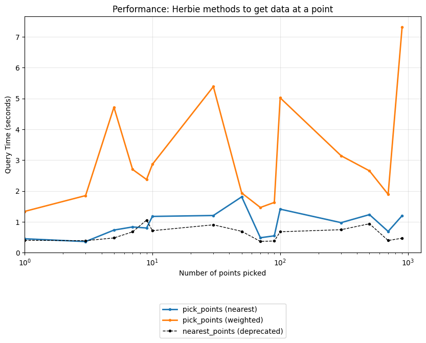
Nice! This BallTree method used by pick_points() scales well for harvesting many points 😎
Lets see how well this works for the GFS model…
[27]:
gfs = Herbie("2024-01-01", model="gfs").xarray(":TMP:2 m ")
✅ Found ┊ model=gfs ┊ product=pgrb2.0p25 ┊ 2024-Jan-01 00:00 UTC F00 ┊ GRIB2 @ aws ┊ IDX @ local
[28]:
%%time
gfs.herbie.pick_points(points_self)
---------------------------------------------------------------------------
NameError                                 Traceback (most recent call last)
File <timed eval>:1

NameError: name 'points_self' is not defined
Advanced Options#
The default behavior for method='nearest' is to return the first nearest neighbor. The default behavior for method='weighted' is to return the inverse-distance weighted mean of the nearest 4 grid points.
You can get more or fewer neighbors by setting the k argument. This might be useful if you want to compute the standard deviation of the k grid points surrounding a point of interest.
[29]:
%%time

# Return the 5 nearest grid points to each request point
ds.herbie.pick_points(points_self_100, method="nearest", k=5)
CPU times: user 2.13 s, sys: 819 ms, total: 2.95 s
Wall time: 2.96 s
[29]:
<xarray.Dataset> Size: 24kB
Dimensions:              (k: 5, isobaricInhPa: 5, point: 100)
Coordinates:
    time                 datetime64[ns] 8B 2024-03-28
    step                 timedelta64[ns] 8B 00:00:00
  * isobaricInhPa        (isobaricInhPa) float64 40B 1e+03 925.0 ... 700.0 500.0
    latitude             (k, point) float64 4kB 29.72 26.96 47.38 ... 35.9 45.11
    longitude            (k, point) float64 4kB 274.8 255.3 ... 285.7 294.9
    valid_time           datetime64[ns] 8B 2024-03-28
    gribfile_projection  object 8B None
    point_grid_distance  (k, point) float64 4kB 0.0 0.0 0.0 ... 2.997 2.979
    point_latitude       (point) float64 800B 29.72 26.96 47.38 ... 35.88 45.14
    point_longitude      (point) float64 800B 274.8 255.3 258.4 ... 285.7 294.9
    point_stid           (point) object 800B 'SkNxqxCY' ... 'KYvNRgCr'
Dimensions without coordinates: k, point
Data variables:
    t                    (k, isobaricInhPa, point) float32 10kB 293.1 ... 259.9
Attributes:
    GRIB_edition:            2
    GRIB_centre:             kwbc
    GRIB_centreDescription:  US National Weather Service - NCEP
    GRIB_subCentre:          0
    Conventions:             CF-1.7
    institution:             US National Weather Service - NCEP
    model:                   hrrr
    product:                 sfc
    description:             High-Resolution Rapid Refresh - CONUS
    remote_grib:             https://noaa-hrrr-bdp-pds.s3.amazonaws.com/hrrr....
    local_grib:              /home/blaylock/data/hrrr/20240328/subset_0befe27...
search: TMP:\d* mb[30]:
%%time
# Compute the distance weighted mean for the 9 nearest grid points to
# each request point
ds.herbie.pick_points(points_self_100, method="weighted", k=9)
CPU times: user 3.12 s, sys: 341 ms, total: 3.46 s
Wall time: 3.5 s
[30]:
<xarray.Dataset> Size: 28kB
Dimensions:              (isobaricInhPa: 5, point: 100, k: 9)
Coordinates:
    time                 datetime64[ns] 8B 2024-03-28
    step                 timedelta64[ns] 8B 00:00:00
  * isobaricInhPa        (isobaricInhPa) float64 40B 1e+03 925.0 ... 700.0 500.0
    valid_time           datetime64[ns] 8B 2024-03-28
    gribfile_projection  object 8B None
    point_latitude       (point) float64 800B 29.72 26.96 47.38 ... 35.88 45.14
    point_longitude      (point) float64 800B 274.8 255.3 258.4 ... 285.7 294.9
    point_stid           (point) object 800B 'SkNxqxCY' ... 'KYvNRgCr'
    latitude             (k, point) float64 7kB 29.72 26.96 47.38 ... 35.91 45.1
    longitude            (k, point) float64 7kB 274.8 255.3 ... 285.6 294.9
    point_grid_distance  (k, point) float64 7kB 0.0 0.0 0.0 ... 4.238 4.213
Dimensions without coordinates: point, k
Data variables:
    t                    (isobaricInhPa, point) float64 4kB 293.1 ... 259.8
Attributes:
    pick_point_method:  weighted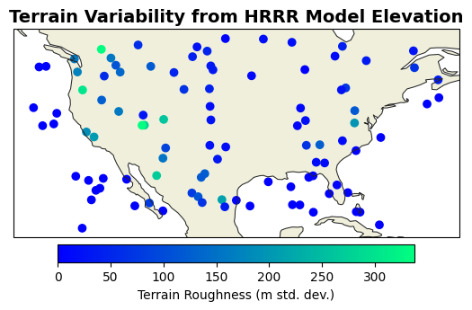
pick_point_k: 9Suppose I wanted to calculate terrain roughness around each point using k-nearest neighbors by calculating the standard deviation of model surface height around each of my points.
[31]:
ds = Herbie("2024-01-01").xarray("HGT:surface")
dsp = ds.herbie.pick_points(points_self_100, k=100)
dsp
✅ Found ┊ model=hrrr ┊ product=sfc ┊ 2024-Jan-01 00:00 UTC F00 ┊ GRIB2 @ aws ┊ IDX @ local
[31]:
<xarray.Dataset> Size: 282kB
Dimensions:              (k: 100, point: 100)
Coordinates:
    time                 datetime64[ns] 8B 2024-01-01
    step                 timedelta64[ns] 8B 00:00:00
    surface              float64 8B 0.0
    latitude             (k, point) float64 80kB 29.72 26.96 ... 35.96 45.07
    longitude            (k, point) float64 80kB 274.8 255.3 ... 285.8 294.7
    valid_time           datetime64[ns] 8B 2024-01-01
    gribfile_projection  object 8B None
    point_grid_distance  (k, point) float64 80kB 0.0 0.0 0.0 ... 16.95 16.85
    point_latitude       (point) float64 800B 29.72 26.96 47.38 ... 35.88 45.14
    point_longitude      (point) float64 800B 274.8 255.3 258.4 ... 285.7 294.9
    point_stid           (point) object 800B 'SkNxqxCY' ... 'KYvNRgCr'
Dimensions without coordinates: k, point
Data variables:
    orog                 (k, point) float32 40kB 6.263 1.444e+03 ... 0.01339
Attributes:
    GRIB_edition:            2
    GRIB_centre:             kwbc
    GRIB_centreDescription:  US National Weather Service - NCEP
    GRIB_subCentre:          0
    Conventions:             CF-1.7
    institution:             US National Weather Service - NCEP
    model:                   hrrr
    product:                 sfc
    description:             High-Resolution Rapid Refresh - CONUS
    remote_grib:             https://noaa-hrrr-bdp-pds.s3.amazonaws.com/hrrr....
    local_grib:              /home/blaylock/data/hrrr/20240101/subset_6bef832...
search: HGT:surface[32]:
terrain_roughness = dsp.orog.std(dim="k")
terrain_roughness
[32]:
<xarray.DataArray 'orog' (point: 100)> Size: 400B
array([3.74864864e+00, 7.70284042e+01, 3.17707424e+01, 1.59296356e+02,
       8.50554657e+00, 2.69303436e+02, 2.61035797e+02, 0.00000000e+00,
       7.76310120e+01, 1.48034021e-02, 3.39158669e+01, 1.53166565e+02,
       1.60940230e+00, 0.00000000e+00, 7.13127975e+01, 1.51575775e+01,
       6.64364319e+01, 0.00000000e+00, 1.12974800e+02, 0.00000000e+00,
       2.69054890e+00, 0.00000000e+00, 3.99752159e+01, 3.41971703e+01,
       6.46535950e+01, 3.35994232e+02, 1.60176880e+02, 1.26123024e+02,
       0.00000000e+00, 0.00000000e+00, 0.00000000e+00, 9.03021851e+01,
       1.89539986e+01, 0.00000000e+00, 4.04688110e+01, 0.00000000e+00,
       0.00000000e+00, 4.26026802e+01, 0.00000000e+00, 6.81077968e-03,
       1.19178711e+02, 2.45614243e+01, 0.00000000e+00, 6.05588112e+01,
       1.23778839e+02, 1.43709764e+01, 1.18544037e+02, 1.87431240e+01,
       2.04521179e+02, 1.97443123e+01, 1.72476761e+02, 9.15527344e-05,
       0.00000000e+00, 1.38174944e+01, 2.12805542e+02, 2.74857578e+01,
       1.04479446e+01, 1.16316414e+02, 1.93214893e+01, 6.84824142e+01,
       1.96816833e+02, 5.76621933e+01, 0.00000000e+00, 2.23715057e+01,
       0.00000000e+00, 0.00000000e+00, 1.37994690e+02, 2.15656357e+01,
       5.08315516e+00, 0.00000000e+00, 0.00000000e+00, 3.51489334e+01,
       1.04980412e+01, 0.00000000e+00, 2.73795258e+02, 3.37753448e+02,
       1.87713989e+02, 2.93994026e+01, 0.00000000e+00, 0.00000000e+00,
       2.48333950e+01, 1.72831936e+01, 3.04587769e+02, 4.41159105e+00,
       2.12090187e+01, 4.74487686e+01, 1.65152624e-01, 0.00000000e+00,
       0.00000000e+00, 1.64283066e+01, 1.11062164e+02, 0.00000000e+00,
       4.81408958e+01, 0.00000000e+00, 1.59145447e+02, 1.24982613e+02,
       6.93545532e+01, 0.00000000e+00, 0.00000000e+00, 3.61904716e+01],
      dtype=float32)
Coordinates:
    time                 datetime64[ns] 8B 2024-01-01
    step                 timedelta64[ns] 8B 00:00:00
    surface              float64 8B 0.0
    valid_time           datetime64[ns] 8B 2024-01-01
    gribfile_projection  object 8B None
    point_latitude       (point) float64 800B 29.72 26.96 47.38 ... 35.88 45.14
    point_longitude      (point) float64 800B 274.8 255.3 258.4 ... 285.7 294.9
    point_stid           (point) object 800B 'SkNxqxCY' ... 'KYvNRgCr'
Dimensions without coordinates: point[35]:
ax = EasyMap().LAND().ax

art = ax.scatter(
    terrain_roughness.point_longitude,
    terrain_roughness.point_latitude,
    c=terrain_roughness,
    cmap="winter",
)
plt.colorbar(
    art,
    ax=ax,
    label="Terrain Roughness (m std. dev.)",
    orientation="horizontal",
    pad=0.02,
    shrink=0.8,
)

ax.set_title(
    "Terrain Variability from HRRR Model Elevation", fontsize=14, fontweight="bold"
)
[35]:
Text(0.5, 1.0, 'Terrain Variability from HRRR Model Elevation')